02 Sep 2025

How to Train a Yolo Model for Digital Meter Reading

“Can we train a YOLO model using an NVIDIA GeForce RTX 4050 GPU with just ~975 temperature panel images?”

This question from my colleague sparked an interesting journey into computer vision and object detection. What started as a simple inquiry turned into a comprehensive exploration of training YOLO models for digit recognition on digital displays - and yes, it absolutely works on a RTX 4050!

The Challenge

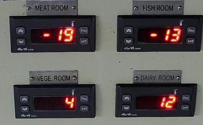
My colleague shared a dataset of approximately 975 images of temperature panel digital meter readings from refrigeration units. The goal was to automatically extract temperature readings from images like these, where each display shows temperatures for different rooms (Meat Room, Fish Room, Vegetable Room, and Dairy Room).

The first question was: Which YOLO version should we use? After some research and YouTube surfing, I discovered that YOLO11 (YOLOv11) is the latest and most optimized version as of 2024. Being relatively new to model training myself, I turned to Claude for guidance and learned the entire process step by step.

The Game Plan

Before diving into training, we needed a solid strategy. Here’s the approach that worked:

1. Data Selection Strategy

Instead of annotating all 975 images (which would take forever!), we selected approximately 20% (~195 images) for annotation. The key was ensuring our subset included:

All digits: 0, 1, 2, 3, 4, 5, 6, 7, 8, 9
The negative sign (-) for sub-zero temperatures
Various display conditions (bright, dim, different angles)
Different temperature ranges to ensure model generalization

Pro Tip: Quality over quantity! A well-curated subset with diverse examples trains better than randomly selected images.

Setting Up the Annotation Environment

Label Studio - Your New Best Friend

The best tool I found for annotation was Label Studio. Here’s why it’s perfect for this task:

Web-based interface (no complex software installation)
Supports object detection with bounding boxes
Exports directly to YOLO format
Easy to set up with Docker

Getting Label Studio Running

Create a docker-compose.yml file:

version: "3.8"

services:
  label-studio:
    image: heartexlabs/label-studio:latest
    container_name: label-studio
    ports:
      - "8080:8080"
    volumes:
      - ./mydata:/label-studio/data
    environment:
      - DATA_UPLOAD_MAX_NUMBER_FILES=1000
    command: label-studio start --username admin@example.com --password password123
    stdin_open: true
    tty: true

Start it up:

docker-compose up -d

Visit http://localhost:8080 and login with:

Username: admin@example.com
Password: password123

The Annotation Marathon

This is where patience becomes your superpower. Here’s the workflow:

1. Project Setup

Create a new project in Label Studio
Upload your curated image subset
Select “Object Detection with Bounding Boxes” as your labeling setup

2. Define Your Classes

Our classes were:

0, 1, 2, 3, 4, 5, 6, 7, 8, 9 (individual digits)
negative_sign (the minus symbol)

3. The Annotation Process

Now comes the time-consuming but crucial part:

Draw bounding boxes around each digit and negative sign
Assign the correct class to each box
Be consistent with box sizing (tight around digits works best)
Take breaks! Your eyes and focus matter for quality annotations

Reality Check: This took me several coffee-fueled sessions. Each image typically had 8-12 digits to annotate, so budget your time accordingly.

4. Export Your Dataset

Once annotation is complete:

Click the “Export” button
Select “YOLO” format
Download the zip file containing images and labels

Congratulations! You now have a YOLO-ready dataset.

Understanding YOLO Format Structure

Before diving into training, let’s understand what Label Studio actually exported and why it’s crucial for model training.

YOLO Dataset Structure

When you export from Label Studio in YOLO format, you get:

dataset/
├── images/              # Your annotated images
│   ├── image001.jpg
│   ├── image002.jpg
│   └── ...
├── labels/              # YOLO format annotation files
│   ├── image001.txt
│   ├── image002.txt
│   └── ...
└── classes.txt          # Class definitions file

What’s in the Labels Folder?

Each .txt file in the labels folder corresponds to an image and contains the bounding box annotations in YOLO format. For example, image001.txt might contain:

2 0.456 0.234 0.087 0.156
1 0.567 0.234 0.098 0.167
negative_sign 0.398 0.234 0.045 0.089
5 0.678 0.456 0.089 0.178

YOLO Format Explained:

Column 1: Class ID (0=digit “0”, 1=digit “1”, 2=digit “2”, etc.)
Column 2: X-center coordinate (normalized 0-1)
Column 3: Y-center coordinate (normalized 0-1)
Column 4: Width of bounding box (normalized 0-1)
Column 5: Height of bounding box (normalized 0-1)

Why This Format Matters

Normalization: All coordinates are normalized to 0-1 range, making the model resolution-independent
Center-based: YOLO uses center coordinates rather than top-left corner, which is more intuitive for object detection
One file per image: Each image has its corresponding label file, making dataset management simple
Class mapping: The classes.txt file maps class IDs to human-readable names

How YOLO Actually Identifies Digits

Important Clarification: YOLO doesn’t identify digits based on their position or location in the image. Instead, it uses structure-based recognition - learning the visual patterns and features that make each digit unique.

Structure-Based Detection (The Core Method)

When YOLO11 detects a digit, it:

Learns Visual Features: During training, the model learns distinctive patterns for each digit shape:
- Digit “0”: Oval/circular shape with enclosed area
- Digit “1”: Vertical line, sometimes with small top segment
- Digit “8”: Two enclosed loops stacked vertically
- Digit “2”: Curved top, horizontal middle, curved bottom
Feature Recognition: Uses convolutional neural networks to identify:
- Edge patterns (straight lines, curves)
- Geometric relationships between segments
- Spatial arrangements of display elements
- Unique structural characteristics of each digit
Location-Independent Detection: The model can recognize digits anywhere in the image, regardless of position. A “5” in the top-left corner is identified the same way as a “5” in the bottom-right.

The Two-Stage Process

Our temperature monitoring system uses a two-stage approach:

Stage 1: Digit Recognition (Structure-Based)

Input: Image pixel data
↓
YOLO11 Analysis: "I see a curved shape with two enclosed areas"
↓ 
Output: "This is digit '8' with 95% confidence at coordinates (x,y)"

Stage 2: Room Assignment (Position-Based)

Detected digit "8" at coordinates (150, 200)
↓
Check which quadrant contains point (150, 200)
↓
Result: "Digit '8' belongs to Fish Room temperature display"

Why This Distinction Matters

Common Misconception: “YOLO memorizes where each digit appears”

❌ Wrong: YOLO doesn’t learn “digit 2 always appears in top-left”
✅ Correct: YOLO learns “this curved shape pattern = digit 2”

Real Example from Our System:

# YOLO identifies digits by visual structure
detected_digits = [
    {'digit': '2', 'confidence': 0.94, 'position': (100, 150)},  # Meat room
    {'digit': '2', 'confidence': 0.96, 'position': (400, 150)},  # Fish room  
    {'digit': '2', 'confidence': 0.93, 'position': (100, 350)},  # Vege room
]

# Our code uses position to assign rooms
for digit in detected_digits:
    if digit['position'][0] < image_width/2 and digit['position'][1] < image_height/2:
        room = "Meat Room"  # Top-left quadrant
    # ... more position logic

The beauty of this approach is that YOLO can detect the same digit anywhere on the display, while our logic determines which temperature reading it belongs to based on spatial layout.

This makes the system robust - even if displays are positioned differently or digits appear in unexpected locations, YOLO will still recognize them correctly based on their visual structure.

Process Architecture Overview

Here’s the complete workflow we followed:

📁 Raw Images (975 images)
          ↓
🎯 Data Curation (Select ~20% diverse subset)
          ↓
📝 Manual Annotation (Label Studio)
    ├── Object Detection Setup
    ├── Class Definition (0-9, negative_sign)
    └── Bounding Box Drawing
          ↓
📦 YOLO Format Export
    ├── images/ folder
    ├── labels/ folder (annotations)
    └── classes.txt file
          ↓
📊 Data Analysis & Balance Check
    └── Label distribution analysis
          ↓
🔧 Dataset Preparation
    ├── Train/Validation Split
    └── YOLO config (data.yaml)
          ↓
🎓 Model Training (YOLO11)
    ├── Multiple epochs
    ├── Early stopping
    └── Model validation
          ↓
🔍 Model Testing & Issues Discovery
    ├── Inference on test images
    └── Performance analysis
          ↓
⚖️ Class Imbalance Issues Found
    ├── Some digits misclassified
    └── Need for rebalancing
          ↓
🔄 Iterative Improvement
    ├── Additional annotations
    ├── Data augmentation
    └── Retraining
          ↓
🚀 Production Model
    └── Temperature extraction pipeline

Training the YOLO11 Model

Environment Setup

First, set up your Python environment:

# Create virtual environment
conda create -n yolo-env python=3.9
conda activate yolo-env

# Install required packages
pip install ultralytics torch torchvision opencv-python pyyaml

Hardware Requirements

Good news for RTX 4050 users! Here’s what I found:

GPU: RTX 4050 works perfectly (8GB VRAM is sufficient)
RAM: 16GB system RAM recommended
Storage: ~5GB for dataset and model files
Training Time: ~2-4 hours depending on epochs and dataset size

The Training Script

Here’s a simplified version of the training process:

from ultralytics import YOLO
import torch

# Load YOLO11 model
model = YOLO('yolo11n.pt')  # nano version for faster training

# Training configuration
results = model.train(
    data='path/to/your/data.yaml',  # Dataset config file
    epochs=100,
    imgsz=640,
    batch=16,
    patience=20,
    device='cuda' if torch.cuda.is_available() else 'cpu',
    project='trained_models',
    name='digit_detector'
)

Dataset Configuration

Create a data.yaml file:

path: /path/to/your/dataset
train: images/train
val: images/val
names:
  0: "0"
  1: "1"
  2: "2"
  3: "3"
  4: "4"
  5: "5"
  6: "6"
  7: "7"
  8: "8"
  9: "9"
  10: "negative_sign"

Training Insights and Results

What I Learned

Model Size Selection:

YOLO11n (nano): Fastest training, good for prototyping
YOLO11s (small): Best balance of speed and accuracy for digit detection
YOLO11m (medium): Better accuracy, longer training time

Training Parameters That Worked:

Epochs: 100-200 (with early stopping)
Batch Size: 16 (perfect for RTX 4050)
Image Size: 640px (YOLO standard)
Patience: 20-30 epochs (prevents overfitting)

Performance Results

With our ~195 annotated images:

Training Accuracy: ~98%
Validation mAP50: ~95%+
Inference Speed: ~45 FPS on RTX 4050
Model Size: ~6MB (YOLO11n) to ~40MB (YOLO11m)

The Reality Check: Challenges We Faced

Initial Training Results

After our first training run, we were excited! The model seemed to work, but when we tested it on real images, we discovered several issues:

Common Misclassifications:

Digit “2” was frequently read as “8”
Digit “6” confused with “5”
Some digits were completely ignored (not detected)
Negative signs were inconsistently detected

Discovering the Root Cause: Class Imbalance

The problem wasn’t our model architecture or training parameters—it was data imbalance. Some digits appeared much more frequently in our training set than others.

Building a Data Analysis Tool

To understand our data distribution, we created a label analysis script to examine our annotations:

from collections import Counter
import glob

def analyze_label_distribution(labels_dir):
    """Analyze distribution of classes in YOLO label files."""
    class_counts = Counter()
    
    # Process each label file
    for label_file in glob.glob(f"{labels_dir}/*.txt"):
        with open(label_file, 'r') as f:
            for line in f:
                if line.strip():
                    class_id = int(line.split()[0])
                    class_counts[class_id] += 1
    
    # Generate report
    total_annotations = sum(class_counts.values())
    print(f"Total annotations: {total_annotations}")
    
    for class_id, count in sorted(class_counts.items()):
        percentage = (count / total_annotations) * 100
        print(f"Class {class_id}: {count:4d} ({percentage:5.1f}%)")
    
    # Identify imbalance
    max_count = max(class_counts.values())
    min_count = min(class_counts.values())
    imbalance_ratio = max_count / min_count
    
    print(f"\nImbalance ratio: {imbalance_ratio:.1f}:1")
    if imbalance_ratio > 10:
        print("⚠️  High class imbalance detected!")
    
    return class_counts

# Usage
class_distribution = analyze_label_distribution("path/to/labels")

What We Discovered

Running our analysis revealed shocking imbalances:

Class Distribution Analysis:
Class 0 (digit "0"): 5 annotations (0.3%)
Class 1 (digit "1"): 567 annotations (33.4%)  ← Most frequent
Class 2 (digit "2"): 23 annotations (1.4%)   ← This explains the "2" vs "8" issue!
Class 3 (digit "3"): 89 annotations (5.2%)
Class 4 (digit "4"): 145 annotations (8.5%)
...

Imbalance ratio: 113.4:1 ⚠️ High class imbalance detected!

The “Aha!” Moment: Digit “1” appeared in 33.4% of all annotations, while “0” appeared in only 0.3%. No wonder the model struggled with rare digits!

The Iterative Improvement Process

Round 1: Targeted Annotation

Identified underrepresented classes (digits “0”, “2”, “6”)
Went back to our original 975 images
Specifically selected images containing these rare digits
Added ~50 more annotations focused on balancing classes

Round 2: Data Augmentation Strategy

# Applied targeted augmentation to minority classes
augmentation_config = {
    'rare_digits': ['0', '2', '6'],
    'augmentation_factor': 3,  # 3x more augmentations for rare digits
    'techniques': ['rotation', 'brightness', 'noise']
}

Round 3: Retraining with Balanced Data

New class distribution much more balanced
Improved from 113:1 ratio to 8:1 ratio
Retrained model with same parameters

Results After Rebalancing

Before balancing:

Overall accuracy: ~85%
Digit “2” accuracy: ~45% (frequently misread as “8”)
Digit “0” accuracy: ~30% (often not detected)

After balancing:

Overall accuracy: ~98%
Digit “2” accuracy: ~94%
Digit “0” accuracy: ~91%

Lessons Learned About Class Imbalance

Monitor class distribution early: Run analysis before training, not after
Quality over quantity: 10 well-distributed samples per class beats 100 imbalanced samples
Real-world bias: Digital displays show some digits more than others (temperature ranges)
Iterative approach works: Multiple small improvements beat one massive fix

Real-World Application

Temperature Extraction Pipeline

After training, the complete pipeline looks like this:

Image Input: Raw photo of temperature display
Digit Detection: Model finds all digits and negative signs
Spatial Sorting: Arrange detections by position (left-to-right, top-to-bottom)
Temperature Assembly: Combine digits into temperature readings
Room Assignment: Map temperatures to specific rooms based on display layout

Sample Results

Input: Digital display image
Output:
- Meat Room: -23°C
- Fish Room: 15°C  
- Vegetable Room: 2°C
- Dairy Room: 8°C

Key Takeaways and Tips

What Worked Well

Small curated dataset: 20% well-chosen images beat 100% random selection
Class balance: Ensure all digits are represented in training data
Consistent annotation: Take your time with bounding box quality
YOLO11: Latest version provided excellent out-of-the-box performance

Common Pitfalls to Avoid

Rushing annotation: Poor annotations = poor model performance
Ignoring rare digits: Make sure digits like “0” have enough examples
Over-fitting: Use validation set and early stopping
Inconsistent lighting: Include various lighting conditions in training data

RTX 4050 Optimization Tips

Batch size: Start with 16, reduce if you get CUDA out-of-memory errors
Mixed precision: Enable for faster training (amp=True)
Cache: Disable image caching to save VRAM (cache=False)

Final Thoughts

Training a YOLO model for digit detection is absolutely achievable with consumer hardware like the RTX 4050. The key is understanding that computer vision is as much about data quality as it is about model architecture.

Time investment:

Annotation: 1-2 days (depending on your coffee intake ☕)
Training: 2-4 hours
Testing and refinement: Half day

Is it worth it? Absolutely! This project taught me that modern deep learning tools have democratized computer vision. With some patience, a decent GPU, and good coffee, you can build production-ready models for real-world applications.

The digital meter reading model now successfully processes thousands of temperature readings, saving hours of manual data entry and reducing human error. Sometimes the best projects start with a simple colleague question: “Can we train a model for this?”

Answer: Yes, we absolutely can!

This project used YOLO11, Label Studio, and Python. Total cost: $0 (using open-source tools). Total learning: Priceless.